Research Overview
In this part of the web page I want to present part of my research.
I try to summarize the main ideas behind all techniques I use and try to give appropriate references and to sketch how I combine these techniques to arrive at efficient computational tools for use in Theoretical Chemistry.
Automated Workflows for Quantum Chemical Calculations
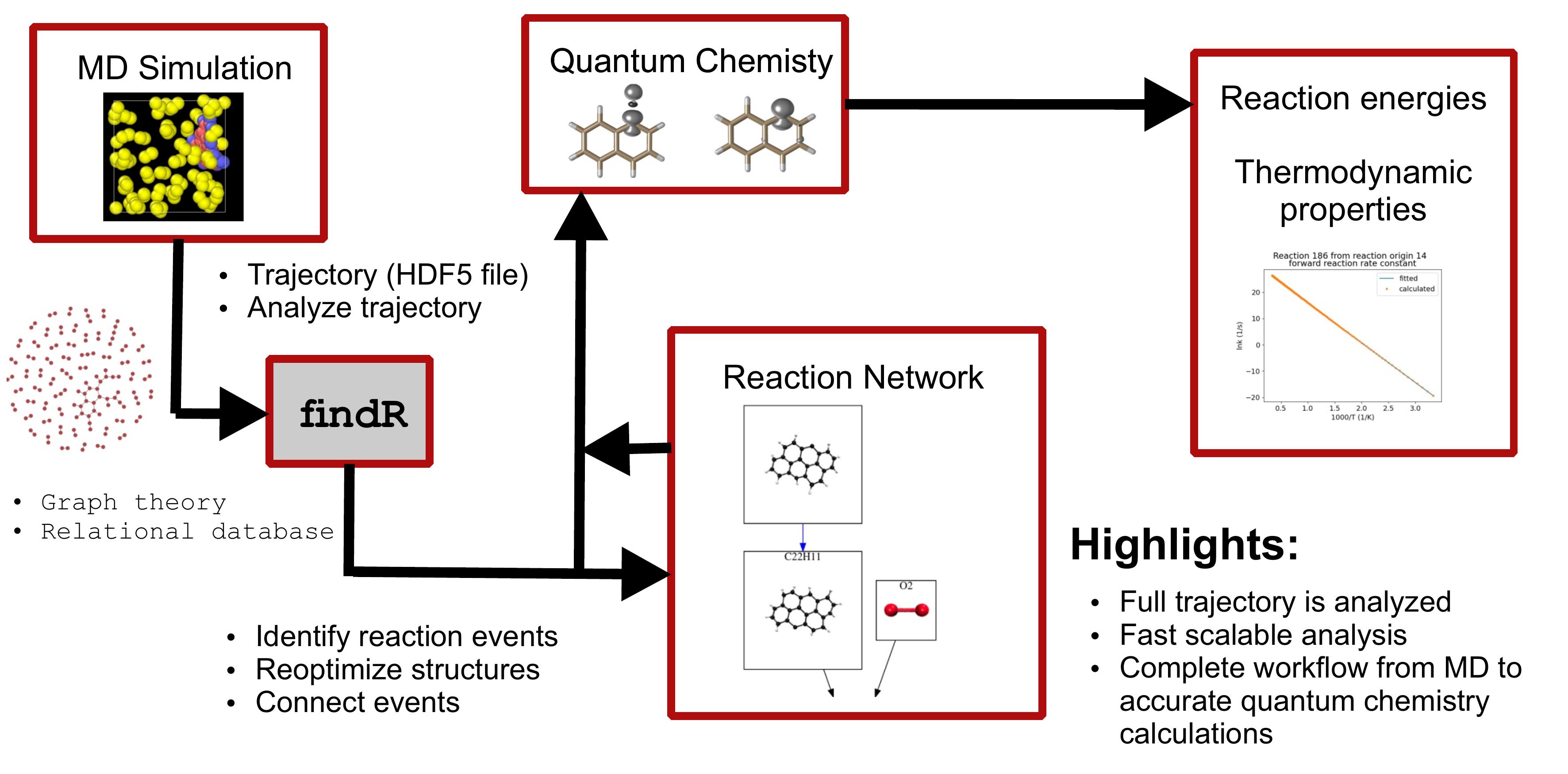
Over the last decades quantum chemical methods have become an important tool for general chemical research since they enable us to interpret experimental data and provide data that is not easily accessible by experimental techniques. They can for example play a key role in unveiling reaction mechanisms. However, the chemical reaction space is so large that often relying on chemical (human) intuition is the bottleneck in such a study. Thus, it is important to develop automatized workflows which make for example reaction discovery a self-driven problem. For that purpose we proposed [1] an automatized workflow starting from reactive molecular dynamics simulations (ReaxFF or GFN-xTB) to accurate quantum chemical chemical calcualtions employing DFT and/or Coupled Cluster.
In a long run the work on automatized workflows falls nicely in our work on Machine Learning applications in quantum Chemistry since they are a natural mean to generate well-balanced training sets if combined with ideas of Bayesian optimization to only include points which will yield an information gain.
References
Machine Learning for Chemical Applications
My main work horse for Machine Learning (ML) applications is Gaussian Process Regression (GPR), which I employ to construct potential energy surfaces (PESs) more efficiently. Find below an outline about the theory behind GPR and later how it is used in our setup.
Gaussian Process Regression
Gaussian process regression (GPR), sometimes also referred to as kriging [1-3], belongs to the field of ML algorithms. It has its strength in the non parametric regression of multidimensional hypersurfaces using only limited input data. GPR is based on Bayesian inference [4] and by definition a Gaussian Process (GP) is a statistical distribution of functions, for which every finite linear combination of samples has a joint Gaussian distribution. With the aim to model a potential \(V(x)\) we introduce the vector \({\bf{v}}=\left(V({\bf{x_1}}),V({\bf{x_2}}),...,V({\bf{x_n}})\right)\), where \({\bf{x}}=\left(x_1,x_2,...,x_d\right)\) is also a vector of dimensionality \(d\) containing the coordinates of a given structure (data point). We now assume that the elements of \({\bf{v}}\) follow a multivariant Gaussian distribution, and thus we can write the joint probability density as
or use the short-hand notation
Without loosing generality we assume a zero mean function \({\bf{m}}=\left(m({\bf{x_1}}),m({\bf{x_2}}),...,m({\bf{x_n}})\right) = \mathbf{0}\).
Predictions in GPR are made through inference. We exploit that the observed/training data \(\bf{v}\) and new points of interest \({\bf{v}}_{*}=\left(V({\bf{x_1^{*}}}),V({\bf{x_2^{*}}}),...,V({\bf{x_n^{*}}})\right)\) are distributed according to the same distribution
where \({\bf{X}}=\left( {\bf{x}}_1, {\bf{x}}_2,...,{\bf{x}}_n\right)\) is a vector of the \(n\) data points. By conditioning this joint Gaussian prior distribution on the observations one obtains the Bayesian conditional probability (or posterior distribution)
which is defined by a new mean function and co-variance matrix
The posterior mean is used as predictor and the diagonal of posterior co-variance matrix serves as uncertainty measurement for our predictions.
Since calculations are only done with finite precision and it can add flexibility to the GPR we incorporate a constant noise term \(\sigma^2\) on the diagonal of the co-variance matrix
Incorporating this term all presented working equations remain the same, but this term serves as a regularization. The GPR has not to go through each data point exactly anymore, which can result in a smoother regression.
For Potential Energy Surface Construction
The time dominating costs for GPR is the inversion of the co-variance matrix \(\bf K\), which scales with \(\mathcal O(n^3)\). As usual the inversion can be avoided by solving the linear systems of equations
Since \({\bf{K}}\) is positive definite the Cholesky decomposition is the method of choice due to its efficiency and stability.
The final GPR approximated potential is then expressed as
where \(k({\bf{x}}, {\bf{x}}_k)\) is a so called kernel function. The kernel function specifies the co-variance matrix
which is constructed from kernel functions and encodes the closeness of two data points. In our work we usually make use of the Matérn Kernel family
where \(\Gamma\) is the gamma function and \(K_{\nu}\) the modified Bessel function. For half integer values of \(\nu\) some special cases are obtained. In the following the most prominent cases are discussed. For \(\nu=0\) we get the Ornstein-Uhlenbeck kernel (OUEXP)
and for \(\nu = 3/2\) the Matérn 3/2 kernel (MAT32)
and for \(\nu = 5/2\) Matérn 5/2 kernel (MAT52)
Furthermore for \(\lim\nu\rightarrow \infty\) the squared exponential kernel (SQEXP)
is obtained. As a rule of thumb for this class of kernel functions the ability to describe smoother and smoother functions increases with \(\nu\).[4] The kernel function encode the assumed correlation between the data points \({\bf{x}}\) and \({\bf{x}}'\), which are in our case a vector of internal coordinates \({\bf{x}}=(q_1,q_2,...,q_n)^{T}\). There are many more choices for kernel functions and in principle the only crucial requirement is positive definiteness. We note that different kernel functions can for example be combined by addition or multiplication to yield new kernel functions. Multiplication can be seen as an and operation since the new kernel has only high value if both base kernel have high value. Similarly addition can be seen as an or operation. The new kernel has high value if either one or both of the base kernels has high value.
From the definition it is evident that these functions depend on parameters like \(\sigma\) and \(l\). However these parameters are not fit parameters in the classical sense and are therefore usually referred to as hyper parameters. Nevertheless they carry information about the function, which should be described. \(\sigma^2\) is for example the average distance of the function away from its mean and \(l\) is the length of the 'wiggles' in the function. Usually one can not extrapolate more than \(l\) units away from the training data.[4]
Adaptive sampling technique for PES construction exploiting GPR uncertainty
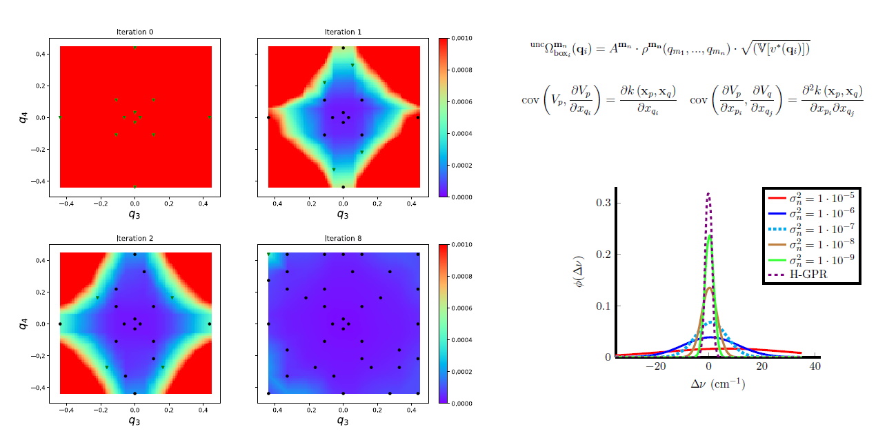
Using GPR we presented a new iterative scheme for potential energy surface (PES) construction, which exploits both physical information and information obtained through statistical analysis. We combined the adaptive density guided approach (ADGA) with GPR, in order to obtain the iterative GPR-ADGA for PES construction. In this new scheme the ADGA provides an average density of vibrational states as a physically motivated importance-weighting and an algorithm for choosing points for electronic structure computations employing this information. GPR is used for an approximation to the full PES given a set of data points. The statistical variance associated with the GPR predictions are used to select the most important points suggested by ADGA. In each iteration the GPR representation of the PES is refined by invoking the ADGA again. Convergence is achieved if no new points in GPR-ADGA are added. Our implementation, additionally, allows for incorporating derivative information in the GPR. The iterative process is started from an initial Hessian and does not require any presampling of configurations prior to the PES construction and thus not additional computational overhead. Comparing PESs obtained by GPR-ADGA and ADGA by calculating fundamental excitation frequencies shows an RMSD below 2 cm\(^{-1}\), while substantial savings of 65-90 % in the number of single point calculations can be achieved.
Extrapolating higher order mode couplings
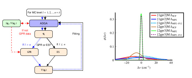
Using GPR we presented a new efficient approach for potential energy surface construction. The algorithm employs the \(n\)-mode representation and combines an adaptive density guided approach with GPRs for constructing approximate higher-order mode potentials.
In this scheme, the \(n\)-mode potential construction is conventionally done, whereas for higher orders the data collected in the preceding steps is used for training in Gaussian Process Regression to infer the energy for new single point computations and to construct the potential.
We explored different delta-learning schemes, which combine electronic structure methods on different levels of theory and found the use of RI-MP2 to target CCSD(F12*)(T) most efficient and also accurate.
Our benchmarks show that for approximate 2-mode potentials the errors can be adjusted to be in the order of 8 cm\(^{-1}\), while for approximate 3-mode and 4-mode potentials the errors fall below 1 cm\(^{-1}\). The observed errors are, therefore, smaller than contributions due to missing higher-order electron excitations or relativistic effects. Most importantly, the approximate potentials are always significantly better than those with neglected higher-order couplings.
Efficient Calculation of Numerical Gradients
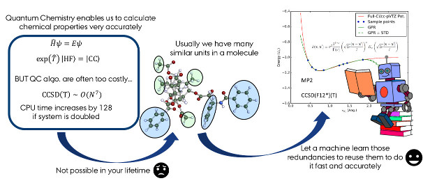
In one of our first studies employing ML techniques we investigated how with means of GPR geometry optimizations, which rely on numerical gradients, can be accelerated. The GPR interpolates a local potential energy surface (PES) on which the structure is optimized.
It is found efficient to combine results on a low computational level (HF or MP2) with the GPR calculated gradient of the difference between the low level method and the target method, which is CCSD(F12*)(T) in this study.
Overall convergence is achieved if both the potential and the geometry is converged. Compared to numerical gradient based algorithms the number of required single point calculations (SPs) is reduced. Although introducing an error due to the interpolation the optimized structures are sufficiently close to the minimum of the target level of theory meaning that the reference and predicted minimum only vary energetically in the \(\mu E_h\) regime.
Low scaling explicitly correlated electronic structure methods
One of the two main problems of wave functions based methods to describe dynamical electron correlation is the steep scaling of computational costs with the system size and the slow basis set convergence. In my work I combined Pair Natural Orbitals (PNOs) for reducing the scaling of the computational methods and F12 Theory to enhance the basis set convergence. In the following you will find an outline on the theory of PNOs and F12 Theory and later it will be demonstrated how these two approaches can be fruitfully combined, where the combined scheme is more than the sum of its parts.
(Hybrid) Pair Natural Orbitals
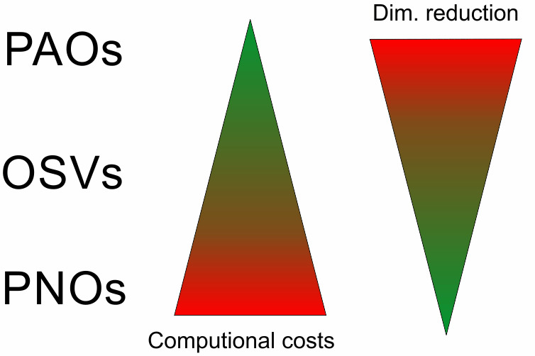
Figure 1. Schematic illustration of relative compression rate and construction cost for PAOs, OSVs and PNOs
PNOs [4-7] are linear combinations of virtual orbitals \(|{a}\rangle\) which are specific for a pair of occupied orbitals \(ij\)
The PNOs are chosen such that they diagonalise the contribution \(D_{ab}^{ij}\) of the pair \(ij\) to the virtual/virtual block of a MP2-like one-electron density matrix:
The eigenvalues \(n_{\bar{a}}^{ij}\) of \(D_{ab}^{ij}\) can be interpreted as the occupation numbers of the PNOs. Sorted in descending order they rapidly decrease to zero. The fast decay allows to truncate the PNO expansion to PNOs with occupation numbers above a threshold \(T_{\rm{PNO}}\) without sacrificing accuracy. The decay is faster if localized occupied orbitals are used.
Deviating from this simple scheme the MP2-like one-electron density is usually build in an already truncated doubles space in order to to avoid the \(\mathcal O(N^5)\) scaling costs for a MP2 calculation.[8-11] For example we use in a hybrid scheme Orbital Specific Virtuals (OSVs) as precursors for the PNOs. They can be seen as the PNOs of the diagonal pairs. The truncation due to the OSVs is coupled to the threshold \(T_{\rm{PNO}}\) to ensure that it does not diminish the overall accuracy. PNOs, OSVs and alternatively projected atomic orbitals (PAOs) are choices for a factorization of the doubles space
All three choices are alternatives to represent the virtual orbital space and in the order PAO, OSV and PNO these representations become more and more compact. However, at increased computational cost for construction as illustrated in Fig. 1.
F12 Theory
Correlated wave function based methods show a slow basis set convergence with respect to the maximal angular momentum \(L\) in a basis. This behavior originates from a cusp in the wave function when two electrons approach each other arbitrarily close at the coalescence point. At this point a singularity in the coulomb interaction of both electrons exists, but since for the exact wave function the local energy at this points remains continuous this singularity has to be canceled by the operator for the kinetic energy. This can be illustrated by the example of a two electron system. The Schrödinger equation for this case has the form:
The nuclear-nuclear interaction \(V_{NN}\) and the nuclear-electron (We assume that the electrons are singulett coupled and not in the nuclei) has a finite value. The singularity in the term \(\frac{1}{r_{12}}\) at \(r_{12}=|\vec{r}_{1}-\vec{r}_{2}|\rightarrow 0\) can only be canceled by the kinetic energy operator to ensure that \(E\) remains finite. However this is only possible if at the coalescence point the wave function is linear in the inter electronic distance \(r_{12}\). Work by Kato [12] lead to the famous cusp condition:
which the exact wave function has to fulfill. As a consequence the leading term in an expansion for the exact wave function must be linear in \(r_{12}\):
The wave function used in conventional methods build from slater determinants does not fulfill this condition, which directly leads to the slow basis set convergence since high angular momenta are required to mimic the cusp approximately. From a mathematical point of view the problem is that we try to expand a function with a discontinuous derivative (with respect to \(r_{12}\)) in functions, which don't have this discontinuity in their derivatives. A similar problem arises if one expands a triangle function in a Fourier series.
From the early days of quantum mechanics wave function Ansätze were known, which didn't have this kind of problems. For example Hylleraas proposed in 1929 the following Ansatz for the wave function of helium
with \(l+m+n\le N\), which has an explicit dependence on the inter electronic distance \(r_{12}\).[13-14] The Hylleraas function shows a significantly improvement of the convergence with the maximal angular momentum. But the Hylleraas Ansatz has the disadvantage that complicates 3 and 4 electron integrals arise, which hamper the application to poly-nuclear systems.
I took quite some time until practical explicitly correlated wave function based methods were proposed. The breakthrough was in 1985 when Kutzelnigg published his ideas which lead to R12- and later to F12-Theory.[15] In R12-Theory as well as the newer F12-Theory the conventional HF orbital basis is augmented by pairfunctions -so called geminals-:
The geminals have via the correlation factor \(f_{12}(r_{12})\) an explicit dependence on the inter electronic distance and are kept orthogonal to the conventional orbital basis with a projector \(\hat{Q}_{12}\), which will be explained in more detail in a subsidiary part.
As indicated in the equation the geminals are constructed from occupied orbitals. It is also possible to additionally construct them from virtual orbitals, but since the occupied orbitals gives the larger contribution this is not done due to efficiency reasons. Due to the cusp condition \(f_{12}(r_{12})\) must fulfill the condition
In R12-Theory only the most important term in the Hylleraas Ansatz is kept, which is linear in \(r_{12}\). The correlation factor is than \(r_{12}(r_{12})\). But in the framework of F12-Theory the correlation factor \(f_{12}(r_{12})=(-\frac{1}{\gamma}\cdot\exp{-\gamma r_{12}})\) is used.[16-17] The exponential factor has the advantage that a larger volume of the cusp can be described, which enhances the accuracy. In most implementations the exponential is approximated by a linear combination of Gaussian, which simplifies the integral evaluation.[17] The parameter \(\gamma\) is a fixed parameter, which is optimized for each basis set and often close to one.
Besides the correlation factor also the choice of the strong orthogonality operator \(\hat{Q}_{12}\) determines the wave function Ansatz. In the literature 3 Ansätze are known:[18]
In the literature the newer version of Ansatz 2 is also known as Ansatz 3, but since it gives the same wave function as Ansatz 2 (old) most authors favor to use the name Ansatz 2. The letters \(O\), \(V\) and \(P\) indicate the projection to the occupied, the virtual and the HF orbital space. The projector for the occupied space is for example defined as
For the other spaces analogue expressions are used.
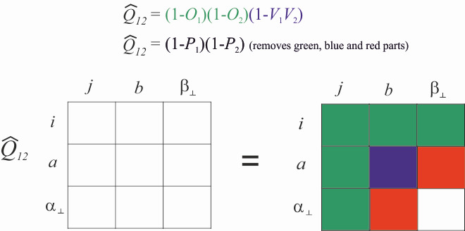
Figure 2. Illustrated action of the orthogonality operator.
Ansatz 1 is not used anymore today or only for higher order terms, since this Ansatz is less accurate than Ansatz 2 (old) and Ansatz 2. The action of \({\hat Q_{12}}\) is depicted in Fig. 2 For a better understanding we introduce a complementary basis \(\{\phi_{\alpha_{\bot}}\}\), which forms with the orbital basis \(\{\phi_{p}\} = \{\phi_{i}\} \cup \{\phi_{a}\}\) a formal complete basis \(\{\phi_{\kappa}\} = \{\phi_{p}\} \cup \{\phi_{\alpha_{\bot}}\}\). The part \(\big( {1 - {{\hat O}_1}} \big)\big( {1 - {{\hat O}_2}} \big)\) removes the parts of the reference determinant as well as single excitations and pauli forbidden excitations (highlighted in green). Only true double excitations remains, where Ansatz 2 with \(\big( {1 - {{\hat V}_1}{{\hat V}_2}} \big)\) also removes the conventional double excitations (highlighted in blue). Ansatz 1 would also remove the parts highlighted in red. If the conventional and explicitly correlated double excitations are not treated differently and no approximations are introduced in the calculations of the matrix elements, Ansatz 2 (old) and Ansatz 2 are equivalent. But since Ansatz 2 ensures that the explicitly correlated double excitations are orthogonal to the conventional ones, the coupling elements between the conventional and explicitly correlated double excitations and the geminals are small, which makes it easier to introduce approximations. For Ansatz 2 (old) the coupling elements do not vanish in the basis set limit and therefore approximations in the calculations in the matrix elements also lead to a different basis set limits. Therefore Ansatz 2 is now standard in modern implementations. Moreover Ansatz 2 (old) also leads for CC methods to numerical problems in the solutions of the CC equations and as a consequence significantly more iterations are needed.
F12 PNOs
When combining PNOs with F12 Theory we can exploit that parts of the virtuals can be described by the geminals in order to reduce the number of required PNOs per pair further. In this spirit PNOs for the virtual space in F12 calculations, F12-PNOs, are obtained from densities build from the differences [19]
between amplitudes \(t^{ij}_{ab}\) for double excitations into products of virtual MOs and the part \(r_{ab}^{\widetilde{ij}}\) that can be described by the geminal \(\chi_{ij}\). Besides the F12-PNOs additional auxiliary PNOs (X-PNOs) have to be introduced in order to arrive at a pair-specific representation of the F12 strong orthogonality operator.[20] These X-PNOs are also truncated according to thresholds, which are automatically adjusted [19] to the value of \(T_{\rm{PNO}}\).
PNO-CCSD(F12*)(T) and its applications
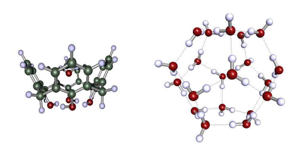
Figure 3. Illustration of host guest systems investigated with PNO-CCSD(F12*)(T)
We used the F12-PNOs for an efficient implementation of PNO-CCSD(F12*)(T) incorporating the Laplace trick to account for the full triples correction.[20-21] With this implementation we were able to calcualte binding energies in large host guest systems and large water complexes as illustrated both in Fig. 3 and Table 1. Furthermore we provided new benchmark data for weak molecular dimer interactions [20-21] and benchmarked PNO-CCSD(F12*)(T) against state of the art methods for obtaining reaction energies [22].
Table 1. Counterpoise corrected \(E^{CP}_{\mathrm{bind}}\) and not corrected \(E_{\mathrm{bind}}\) binding energies for the water molecule in the Calix[4]arene water comples using a PNO threshold of \(T_{\rm{PNO}}=10^{-7}\) and the aug-cc-pVDZ basis.
| Method | \(E^{CP}_{\mathrm{bind}}\) (kcal/mol) | \(E_{\mathrm{bind}}\) (kcal/mol) |
|---|---|---|
| HF | 4.26 | 2.27 |
| PNO-MP2-F12 | -7.72 | -8.50 |
| PNO-SCS-MP2-F12 | -4.95 | -5.70 |
| PNO-CCSD(F12*) | -4.13 | -5.03 |
| PNO-CCSD(F12*)(T0) | -5.16 | -6.56 |
| PNO-CCSD(F12*)(T) | -5.26 | -6.65 |
| PNO-CCSD(F12*)(T*) | -5.60 | -7.02 |
- G.Schmitz, C.Hättig, D.P.Tew, "Explicitly correlated PNO-MP2 and PNO-CCSD and their application to the S66 set and large molecular systems", Phys. Chem. Chem. Phys.,2014,16, 22167-22178.
- G.Schmitz, C.Hättig, "Perturbative triples correction for local pair natural orbital based explicitly correlated CCSD (F12*) using Laplace transformation techniques", The Journal of Chemical Physics,2016,145,234107.
- G.Schmitz, C.Hättig, "Accuracy of explicitly correlated local PNO-CCSD (T)", Journal of Chemical Theory and Computation,2017,13, 2623-2633.
References
- T. L. Fletcher, P. L. A. Popelier, “Multipolar Electrostatic Energy Prediction for all 20 Natural Amino Acids Using Kriging Machine Learning”, Journal of Chemical Theory and Computation 2016, 12, 2742–2751.
- S. M. Kandathil, T. L. Fletcher, Y. Yuan, J. Knowles, P. L. A. Popelier, “Accuracy and tractability of a kriging model of intramolecular polarizable multipolar electrostatics and its application to histidine”, Journal of Computational Chemistry 2013, 34, 1850–1861.
- M. J. L. Mills, P. L. A. Popelier, “Polarisable multipolar electrostatics from the machine learning method Kriging: an application to alanine”, Theoretical Chemistry Accounts 2012, 131, 1137.
- C. E. Rasmussen, C. K. I. Williams, Gaussian Processes for Machine Learning (Adaptive Computation and Machine Learning), The MIT Press, 2005.
- Meyer, W, "Ionization Energies of Water from PNO-CI Calculations" International Journal of Quantum Chemistry 1971, 5, 441–348.
- Ahlrichs, R., Lischka, H., Staemmler, V., Kutzelnigg, W, "PNO-CI (Pair Natural Orbital Configuration Interaction) and CEPA-PNO (Coupled Electron Pair Approximation with Pair Natural Orbitals) Calculations of Molecular Systems. I. Outline of the Method for Closed-Shell States" The Journal of Chemical Physics 1975, 62, 1225.
- Ahlrichs, R., Driessler, F., Lischka, H., Staemmler, V., Kutzelnigg, W, "PNO-CI (Pair Natural Orbital Configuration Interaction) and CEPA-PNO (Coupled Electron Pair Approximation with Pair Natural Orbitals) Calculations of Molecular Systems. II. The Molecules BeH2, BH, BH3, CH4, CH-3, NH3 (Planar and Pyramidal), H2O, OH+3, HF and the Ne Atom" The Journal of Chemical Physics 1975, 62, 1235.
- Hansen, A., Liakos, D. G., Neese, F, "Efficient and Accurate Local Single Reference Correlation Methods for High-Spin Open-Shell Molecules Using Pair Natural Orbitals" The Journal of Chemical Physics 2011, 135, 214102.
- Riplinger, C., Neese, F, "An Efficient and Near Linear Scaling Pair Natural Orbital Based Local Coupled Cluster Method" The Journal of Chemical Physics 2013, 138, 034106.
- Hättig, C., Tew, D. P., Helmich, B, "Local Explicitly Correlated Second- and Third-Oder Møller-Plesset Pertubation Theory with Pair Natural Orbitals" The Journal of Chemical Physics 2012, 136, 204105.
- Werner, H.-J., Knizia, G., Krause, C., Schwilk, M., Dornbach, M. "Scalable Electron Correlation Methods I.: PNO-LMP2 with Linear Scaling in the Molecular Size and Near-Inverse-Linear Scaling in the Number of Processors" Journal of Chemical Theory and Computation 2015, 11, 484–507.
- Kato, T. "On the Eigenfunctions of Many-Particle Systems in Quantum Mechanics" Communications on Pure and Applied Mathematics 10, 151–177 (1957).
- Hylleraas, E. A. "Über den Grundzustand des Heliumatoms" Zeitschrift für Physik 48, 469–494 (1928).
- Hylleraas, E. A. "Neue Berechnung der Energie des Heliums im Grundzustande, sowie des tiefsten Terms von Ortho-Helium" Zeitschrift für Physik 54, 347–366 (1929).
- Kutzelnigg, W. "r12-Dependent Terms in the Wave Function as Closed Sums of Partial Wave Amplitudes for Large l" Theoretica chimica acta 68, 445–469 (1985).
- Ten-no, S. "Initiation of Explicitly Correlated Slater-Type Geminal Theory" Chemical Physics Letters 398, 56–61 (2004).
- Tew, D. P. & Klopper, W. "New Correlation Factors for Explicitly Correlated Electronic Wave Functions" The Journal of chemical physics 123, 074101-074101 (2005).
- Hättig, C., Klopper, W., Köhn, A. & Tew, D. P. "Explicitly Correlated Electrons in Molecules" Chemical Reviews 112, 4–74 (2012).
- Tew, D. P., Hättig, C. Pair Natural Orbitals in "Explicitly Correlated Second-Order Møller-Plesset Theory", International Journal of Quantum Chemistry 113, 224–229 (2013).
- G.Schmitz, C.Hättig, D.P.Tew, "Explicitly correlated PNO-MP2 and PNO-CCSD and their application to the S66 set and large molecular systems", Phys. Chem. Chem. Phys.,2014,16, 22167-22178.
- G.Schmitz, C.Hättig, "Perturbative triples correction for local pair natural orbital based explicitly correlated CCSD (F12*) using Laplace transformation techniques", The Journal of Chemical Physics,2016,145,234107.
- G.Schmitz, C.Hättig, "Accuracy of explicitly correlated local PNO-CCSD (T)", Journal of Chemical Theory and Computation,2017,13, 2623-2633.